Curse of dimensionality part 2: forecast combinations

In a previous post we discussed the term ‘curse of dimensionality’ and showed how it manifests itself, in practice. Here we give another such example.

Forecast combinations

Here is another situation where the ‘curse of dimensionality’ morph an excellent idea in small dimension into an impossible one when dimension is increased. Say you aim to forecast a variable y using possible 10 explanatory variables. An idea is to create a set of forecasts using all possible subsets of those 10 variables. If you create this forecasts using a regression this would be called complete-subset-regressions. This idea is useful on two counts at least.

The first: Graham, Gargano and Timmermann (2013) show that combining all those forecasts is better than trying to identify the best subset. Also they show that the performance is very competitive with other forecast combinations methods. On a close look, the reason is that this kind of forecast combination accounts for the covariance between the explanatory variables. Recall that when using linear regression, the forecasts is simply a linear function of those explanatories, so combining the resulting forecasts means combining a linear function of the explanatories, hence the relation.

The second: complete-subset-regressions is also sometimes used as the basis for the now popular Bayesian model averaging. If you assume normality in the data, you can interpret how close the forecast from some particular subset to the actual observation. From that you can conclude something about the subset and about the explanatory variables that are included in that subset. If a specific variable increases the fit every time it is included, there is a high probability that it is a variable which belongs to the “real” subset (which we don’t know of course).

An easy, simple and intuitive advancement, what else can we wish for? But what about implementation?

Regression is quickly performed, but how many regressions do we need? For 3 explanatory variables we have 7 regressions in total:
3 regressions (each variable separately) + 3 (each two out of the three) + 1 (all three included) = 7.
No problemo.

More generally, for P explanatory variables we have the following formula for $\Psi$ , the number of regressions needed:

(1) $\begin{equation*} \Psi = \sum_{i = 1}^P {{P}\choose{i}} = \sum_{p = 1}^P \frac{P!}{i! (P-i)!} \end{equation*}$

The following figure shows $\Psi$ for when we have 10 variables, and for when we double this number to 20. The blue line indexed 1 is basically 11, index 2 is 12 and so forth.

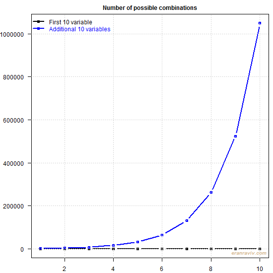
You can see that if you have below say about 13 variables, computation would be rather cheap. However, each additional variables weighs in, and weighs in heavily indeed. Reaching 30 variables would require heavyweight parallel computing which would take days. That is a real shame given how useful is this idea is. Nowadays 20 variables is nothing extraordinary mind you.

There are ways around this issue to some extent but:
(1) they are computationally expensive,
(2) they are only approximations and
(3) they also meet their limits quite quickly.

A valuable idea which, when we try to take advantage of, is being bogged down by curse of dimensionality.

References

Elliott, Graham, Gargano, Antonio & Timmermann, Allan (2013). Complete subset regressions. Journal of Econometrics, 177, 357-373. (link)

Code


# Function to compute how many regressions needed 
# as a function of number of variables
hmc <- function(num_variables){
  out<- NULL
  for (i in 1:num_variables){
    out[i] <- choose(num_variables, i)  
    }
  sum(out)
  }