Forecast averaging example

Especially in economics/econometrics, modellers do not believe their models reflect reality as it is. No, the yield curve does NOT follow a three factor Nelson-Siegel model, the relation between a stock and its underlying factors is NOT linear, and volatility does NOT follow a Garch(1,1) process, nor Garch(?,?) for that matter. We simply look at the world, and try to find an apt description of what we see.
A case in point taken from the yield curve literature is the recent progression towards the “shadow rate” modelling approach, which tackles the zero lower bound problem. A class of models which was nowhere to be found before reality dawned on this special level of policy rates. Model development is often dictated not by our understanding mind you, rather by the arrival of new data which does not fit well existing perceptions. This is not to criticize, but to emphasize: models should be globally viewed as approximations. We don’t really realize reality. Some may even go as far as to argue that reality has no underlying model (or data generating process). As Hansen writes in Challenges for econometric model selection:

“models should be viewed as approximations, and econometric theory should take this seriously”

All theory naturally follow the lines of “if this is the process, then we show convergence to the true parameter”. Convergence is important, but that is a big IF there. Whether there is, or there isn’t such a process, such a true model, we don’t know what it is. Again, especially in social sciences. Furthermore still, even if there is a one true DGP, you can bet on it being variable.

This discussion gives rise to combination of models, or when dealing with the future, combination of forecasts. If we don’t know the underlying truth, combining different choices, or different modelling approaches may yields better results. I consider intelligent combination of forecasts to be weakly dominate (at least not worse, often better than) a single choice made a priori. This is in all usually prevailing situations where the true underlying process is unknown or unstable or both.

How does it work?

Let’s generate some fictitious data, and forecast it using 3 different models. Simple regression (OLS), Boosting and Random forest. Once the three forecasts are obtained, we can average them.

 
# The next line load packages needed for the code to run. If you are missing any, install first.
temp <- lapply(c("randomForest", "gbm", "dismo", "quadprog", "quantreg"), library, character.only=T)
# Code generating the data taken from freakonometrics blog. 
# From the post: REGRESSION MODELS, IT’S NOT ONLY ABOUT INTERPRETATION.
TT <- 1000
set.seed(10)
rtf <- function(a1, a2) { sin(a1+a2)/(a1+a2) }
df <- data.frame(x1=(runif(TT, min=1, max=6)), x2=(runif(TT, min=1, max=6)))
dfx1, dfy <- dfm <- rtf(df_newx2)
df_newm+rnorm(TT_out_of_sample,sd=.1)
boost_fhat <-  p_boost(df_newx2)
rf_fhat <- p_rf(df_newx2)
lm_fhat <- p_lm(df_newx2)
# bind the forecast 
mat_fhat <- cbind(boost_fhat, rf_fhat, lm_fhat)
# name the columns
colnames(mat_fhat) <- c("Boosting", "Random Forest", "OLS")
# Define a battery of forecast combination schemes:
FA_schemes <- c("simple", "ols", "robust", "variance based", "cls")
# FA is a function which will be available in the end of the post
# there are better function in the ForecastCombinations package available from CRAN.
# args(FA) 
# Make room for the results:
results <- list()
# Sacrifice the the initial 30 observations as the initial window
# and reestimate new observation arrive
init_window = 30
for(i in 1:length(FA_schemes)){
	results[[i]] <- FA(df_newMSE, digits=4) ), "\n"  ) )
}
# the function prints the MSE of each forecast averaging scheme:
simple :  1.307 
ols :  1.231 
robust :  1.241 
variance based :  1.241 
cls :  1.195 
# let's check what is the MSE of the individual methods:
mat_err <- apply(mat_fhat, 2, function(x) (df_newy_t\widehat{y}_{i,t}tii = 1i=2 i = 4 . You can just take the average of the forecasts: 
      
 Often, though not very intelligent, this simple average performs very well. 

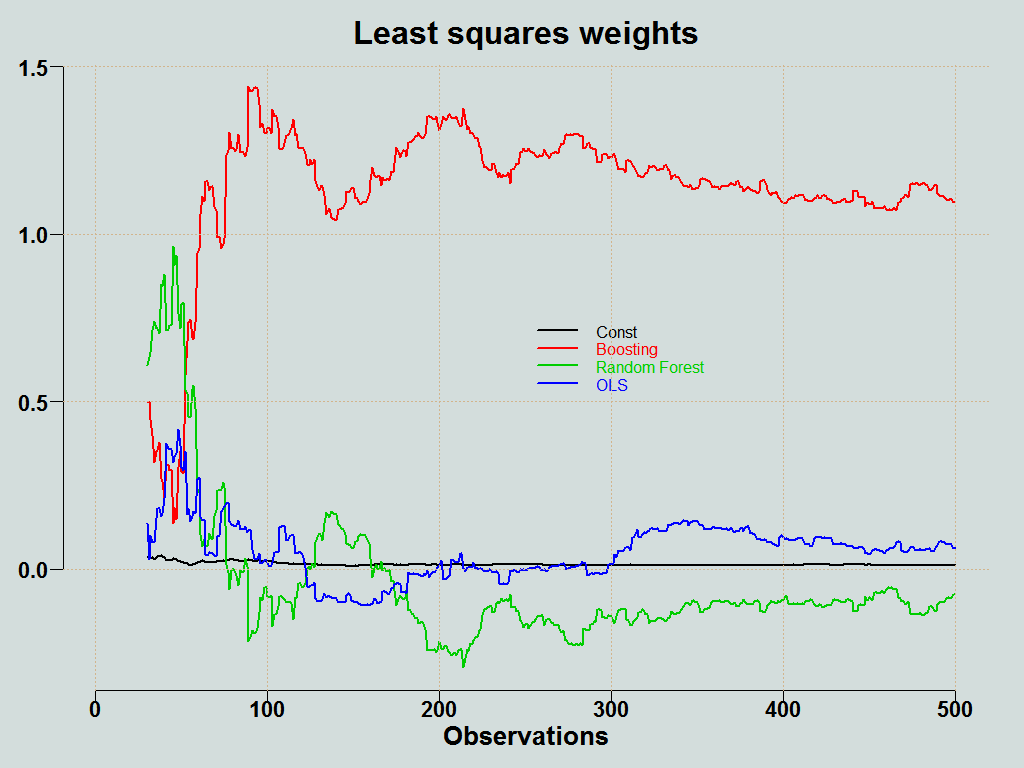
In OLS averaging we simply project the forecast onto the objective, and the resulting coefficients serves as the weights:
      
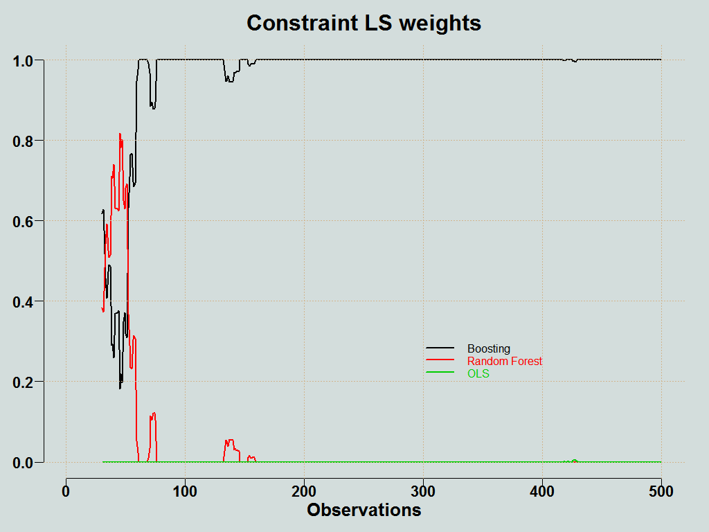
This is quite unstable. All forecasts are chasing the same target, so they are likely to be correlated, which makes it hard to estimate the coefficients. A decent way to stabilize the coefficients is to use constraint optimization, whereby you solve the least squares problem, but under the following constraints:
      

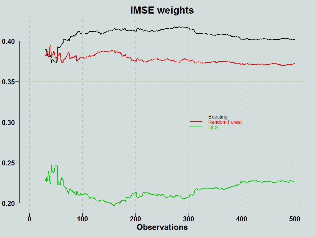
Another way is to average the forecasts according to how accurate they have been, up until that point based on some metric like root MSE. We inverse the weights such that the more accurate (low RMSE) gets more weight:
      

You can plot the weights of the individual methods:






Here is the forecast averaging function (click on the corner arrow to unfold).
# last update: 2015, June. Bug reporting to Eran Raviv
#________________________________________________________________________
FA <- function(obs, mat_fhat, init_window=30,
         Averaging_scheme=c("simple", "ols", "robust", "variance based", "cls", "best")) {
 pckg = c("quantreg", "quadprog")
 temp <- unlist(lapply(pckg, require, character.only=T))
 if (!all(temp==1) ) {
  stop("This function relies on packages \"quadprog\" and \"quantreg\".
Use ?install.packages if they are not yet installed. \n")
 }
 mat_err <- apply(mat_fhat, 2, function(x) obs - x)
 TT <- NROW(mat_fhat)
 p <- NCOL(mat_fhat)
 pred <- NULL
 weights <- matrix(ncol=p, nrow = TT)
 ## Subroutine needed:
 sq_er <- function(obs, pred){ mean( (obs - pred)^2 )  }

 if(length(Averaging_scheme) > 1) {  stop("Pick only one of the following:
 c(\"simple\", \"ols\", \"robust\", \"variance based\", \"cls\", \"best\")") }
 
## Different forecast averaging schemes
## simple
  if(Averaging_scheme=="simple") {
  pred <- apply(mat_fhat, 1, mean)
  weights <- matrix( 1/p, nrow = TT, ncol = p)
  ## OLS weights
    } else if (Averaging_scheme=="ols") {
   weights <- matrix(ncol=(p+1), nrow = TT)   
 for (i in init_window:TT) {
  weights[i,] <- lm(obs[1:(i-1)]~ mat_fhat[1:(i-1),])$coef
 pred[i] <- t(weights[i,])%*%c(1, mat_fhat[i,])
 ## Robust weights
  } } else if (Averaging_scheme=="robust") {
   weights <- matrix(ncol=(p+1), nrow = TT)   
   for (i in init_window:TT) {
    weights[i,] <- rq(obs[1:(i-1)]~ mat_fhat[1:(i-1),])$coef
   pred[i] <- t(weights[i,])%*%c(1, mat_fhat[i,])
   ## Based on the variance of the errors. Inverse of MSE
  } } else if (Averaging_scheme=="variance based") {
  for (i in init_window:TT) {
   temp = apply(mat_err[1:(i-1),]^2,2,mean)/sum(apply(mat_err[1:(i-1),]^2,2,mean))
  weights[i,] <- (1/temp)/sum(1/temp)
  pred[i] <- t(weights[i,])%*%c(mat_fhat[i,])
  ## Using constraint least squares
  }  } else if (Averaging_scheme== "cls") {
   ## Subroutine needed: 
   cls1 = function(y, predictions){
   Rinv <- solve(chol(t(predictions) %*% predictions))
   C <- cbind(rep(1,NCOL(predictions)), diag(NCOL(predictions)))
   b = c(1, rep(0,NCOL(predictions)))
   d = t(y) %*% predictions 
   qp1 = solve.QP(Dmat= Rinv, factorized= TRUE, dvec= d, Amat= C, bvec = b, meq = 1) 
   weights = qp1$sol
   yhatcls = t(weights%*%t(predictions))
   list(yhat= yhatcls, weights= weights)
   }
   ##
for (i in init_window:TT) {
  weights[i,] <- cls1(obs[1:(i-1)], mat_fhat[1:(i-1),])$weights
  pred[i] <- t(weights[i,])%*%c(mat_fhat[i,])
  ## Picking the best performing model up to date according to squared loss function
   } } else if (Averaging_scheme== "best") {
    temp <- apply(mat_fhat[-c(1:init_window),], 2, sq_er, obs= obs[-c(1:init_window)])
    for (i in init_window:TT) {
    weights[i,] <- rep(0,p) 
    weights[i, which.min(temp)] <- 1
    pred[i] <- t(weights[i,])%*%c(mat_fhat[i,])
    } }
 MSE <- sq_er(obs= obs[-c(1:init_window)], pred= pred[-c(1:init_window)])
 return(list(prediction= pred, weights = weights, MSE= MSE))
}

You might also like:
Why complex models are data-hungry?
Correlation and correlation structure (1); quantile regression
Kaggle Experience
Beta in the tails
Subscribe for future posts (no spam)
Like it? share with one click:
Linkedin
Twitter
Email
Facebook
Google
Reddit
Tumblr
Stumbleupon