In multivariate volatility forecasting (4), we saw how to create a covariance matrix which is driven by few principal components, rather than a complete set of tickers. The advantages of using such factor volatility models are plentiful.
First, you don’t model each ticker separately, you can handle tickers with fairly weak liquidity. Second, factor volatility models are computationally cheap. Third, in contrast to exponentially weighted models, the persistence parameter (typically denoted as  ) does not have to be the same across all tickers. You can specify a different process for each of the factors, so that the covariance matrix process enjoys richer dynamics.
No free lunch here though, the cost is a loss of information. It is the cost of condensing the information in the covariance matrix as a whole to just few factors. This means that the factor volatility models are best suited for data that actually display a factor structure (term structures are ideal example). Factor volatility models are not the best choice for data which has weak cross sectional dependence. Too much information is lost in the factorization step.
This post takes us a small step further. We pretty much follow the same methodology presented previously, but now we let the principal components themselves follow a GARCH process. The algebra is fairly simple.
(1) 
with
(2) ![\begin{equation*} \Gamma = [eigenvalue_1 \times \mathbf{eigenvector_i}, ... ,eigenvalue_k \times \mathbf{eigenvector_k} ]. \end{equation*}](https://eranraviv.com/wp-content/ql-cache/quicklatex.com-446cf105fbbfbe6bed4ab18bb662ca63_l3.svg "Rendered by QuickLaTeX.com")
 is a diagonal matrix with dimension as the chosen number of factors. Setting this matrix to be diagonal means that the covariance between the principal components is zero (all off-digaonals elements are zero). Hence they are orthogonal which is the reason for the name*. Of course, by construction the principal components are only unconditionally orthogonal, but we add the constraint\assumption that they are also orthogonal at each point in time. This will ensure the
  is a valid covariance matrix (see part (1) of the series for the meaning of ‘valid’).
The diagonal of is populated with the variance of the factors. Here we use threshold-GARCH model but you can use other process if you want, even as simple as a moving average of the sample variance. What matters is that you keep this matrix diagonal.
Let’s have a look how it works in practice. We use exactly the same data as in the previous post. The four tickers are: ‘IEF’,’TLT’, ‘SPY’, ‘QQQ’. The first two track the short and longer term bond returns, and the last two track some equity indexes. I assume you have the matrix of daily returns, ret, at the ready. See the previous post for code pulling and arranging the data.
The following code is divided into two parts. First, we build our own two factor Orthogonal GARCH model based on a threshold-GARCH model for the individual factors. Use this to better understand the math involved. In the second part we use a package contributed and maintained by Dr. Bernhard Pfaff. Use that for more flexibility in estimation. The package has few different ways to estimate the parameters (non-linear least squares, maximum likelihood and method of moments).
#--------------
# Part one, own specification
#--------------------
library(Matrix) # Douglas Bates and Martin Maechler (2014). Matrix: Sparse and Dense Matrix Classes and Methods. R package version 1.1-3.
library(rugarch) # Alexios Ghalanos (2014). rugarch: Univariate GARCH models. R package version 1.3-4.
# Owing to previous comments, let's keep an out-of-sample perspective
# I use initial window of 1000 observation and re-estimate the parameters of the model with each additional time point
wind <- 1000 #initial window
k <- 2 # number of factors
Uvolatility_fit <- matrix(nrow=(TT), ncol=k) # container of a matrix to hold the volatilities of the three assets
ortgarch <- array(dim = c(TT, l, l)) # make room for your estimate
 ptm <- proc.time() # time the code - it can take a while
 for(i in wind:TT){
pc1 <- prcomp(ret[1:i,], scale. = T) # principal component decomposition
for (j in 1:k){ # for each of the factors same garch process here (but can be different)
Tgjrmodel = ugarchfit(gjrtspec, pc1$x[,j], solver = "hybrid" )
Uvolatility_fit[i,j] =  tail(as.numeric(sigma(Tgjrmodel)),1)
}
w <- matrix(apply(pc1$x, 2, var), nrow = l, ncol = k, byrow = F) *  pc1$rot[,1:k]
# equivalent, more detailed way to obtain w, without using the built in prcomp function:
#--------------
# sret <- scale(ret)
# xpx <- t(sret)%*%sret/(NROW(ret)-1)
# eigval = eigen(xpx, symmetric=T)
# w <- matrix(eigval$values, nrow = l, ncol = k, byrow = F) *  (eigval$vectors)
#--------------
# store the covariance matrices at each point in time:
 for(i in 1:TT){
# This is the Gamma D_t gamma':
ortgarch[i,,] <- w %*% as.matrix(Diagonal(x= (Uvolatility_fit[i,])^2)) %*% t(w)
 }
 proc.time() - ptm
#  user  system elapsed
#  692.63    0.07  693.66 # roughly 12 minutes
#--------------
# # Part two. using Bernhard Pfaff (2012). gogarch: Generalized Orthogonal GARCH (GO-GARCH) models. R package version 0.7-2. (not out-of-sample)
#--------------
library(gogarch)
 Pfaff  <- gogarch(ret,formula = ~garch(1,1), scale = TRUE, estby = "mm")
# other ways to estimate is using ML: estby = "ml", or estby = "nls" which is very fast (type ?gogarch for more)
summary(Pfaff)
slotNames(Pfaff)
# lets get the covariances from this model
myH <- array(dim = dim(ortgarch)) # container with the same dimension as our own ortgarch object
for(i in 1:TT){
	myH[i,,] <- 	Pfaff@H[[i]]
}
# Now let's plot the two. Only the most recent observation, since we used 1000 as initial window
# Change k to denote the most recent observation:
k <- TT - wind
temptime <- tail(time,k) # define the time, (you need code from previous post for the variable time. It's simply the dates of the most recent k returns
# function for plotting the correlation
temp_fun <- function(p1, p2, firstt = F, col, obj = ortgarch){
 	tempcor <- tail(obj[,p1,p2],k)/(tail(sqrt(obj[,p1,p1]),k) * tail(sqrt(obj[,p2,p2]),k))
 	if(firstt){ plot(tempcor~temptime , ty = "l" , ylab = "", ylim = c(-1,1), xlab="")
 		grid()
 		abline(h=0, lty = "dashed", lwd = 2)
 		} else {
 	lines(tempcor~temptime , ty = "l" , col = col) }
 	}
# lets have a look at the resulting correlations:
temp_fun(1,2, col = 1, firstt = T)
temp_fun(1,3, col = 2)
temp_fun(1,4, col = 3)
temp_fun(2,3, col = 4)
temp_fun(2,4, col = 5)
temp_fun(3,4, col = 6)
 title("Own Orthogonal Garch")

 temp_fun(1,2, col = 1, firstt = T, obj = myH)
 temp_fun(1,3, col = 2, obj = myH)
 temp_fun(1,4, col = 3, obj = myH)
 temp_fun(2,3, col = 4, obj = myH)
 temp_fun(2,4, col = 5, obj = myH)
 temp_fun(3,4, col = 6, obj = myH)
title("Orthogonal Garch using the gogarch package")
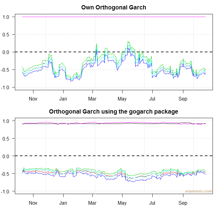
What we see are the six lines corresponding to the 6 correlation series (SPY with TLT, SPY with QQQ etc.). There are few differences between our own estimated model and the one constructed using the gogarch package. But so there should be. Our own specification uses only 2 factors, a difference GARCH model, expanding window for estimation instead of the whole sample, and a different estimation method. I doubt the real correlation are as stable as estimated in the bottom panel. Anyway, this is it. Some references below for the interested reader.
* We mix here terms from algebra, probability and geometry. Orthogonal is a term taken from geometry, and it refers to the angle between two vectors. They are called orthogonal if they are perpendicular. Algebraically, this happens if their inner product  is zero. In probability, coming back to the covariance matrix, COV(x,y) = E(XY) – E(X)E(Y) but because the factors have mean zero: COV(x,y) = E(XY) only. So E(XY) = 0 means that the factors are Orthogonal. Essentially, orthogonality means linear independence.
References
gogarch paper
gogarch package git
A Primer on the Orthogonal GARCH Model (Carol Alexander)
gogarch Presentation (Bernhard Pffaf)


Probably part of the correlation is ‘absorbed’ by the residuals. In other words the principal components are independent (orthogonal) but the residuals are not.