Every form of strength is also a form of weakness*. I love statistics, but I focus to much on methodology, which is not for everyone. Some people (right or wrong) question: “wonderful sir, but what can I do with it?”.
A new paper titled “Beta in the tails” is a showcase application for why we should focus on correlation structure rather than on average correlation. They discuss the question: Do hedge funds hedge? The reply: No, they don’t!
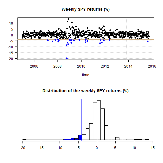
The paper “Beta in the tails” was published in the Journal of Econometrics but you can find a link to a working paper version below. We start with a figure replicated from the paper, go through the meaning and interpretation of it, and explain the methods used thereafter.