5 weeks ago we took a look at the rising volatility in the (US) equity markets via a time-series threshold model for the VIX. The estimate suggested we are crossing (or crossed) to the more volatile regime. Here, taking somewhat different Hidden Markov Model (HMM) approach we gather more corroboration (few online references at the bottom if you are not familiar with HMM models. The word hidden since the state is ‘invisible’).
Category: Blog
Advances in post-model-selection inference (2)
In the previous post we reviewed a way to handle the problem of inference after model selection. I recently read another related paper which goes about this complicated issues from a different angle. The paper titled ‘A significance test for the lasso’ is a real step forward in this area. The authors develop the asymptotic distribution for the coefficients, accounting for the selection step. A description of the tough problem they successfully tackle can be found here.
The usual way to test if variable (say variable j) adds value to your regression is using the F-test. We once compute the regression excluding variable j, and once including variable j. Then we compare the sum of squared errors and we know what is the distribution of the statistic, it is F, or  , depends on your initial assumptions, so F-test or -test. These are by far the most common tests to check if a variable should or should not be included. Problem arises if you search for variable j beforehand.
Advances in post-model-selection inference
Along with improvements in computational power, variable selection has become one of the problems attracting the most effort. We (well.. experts) have made huge leaps in the realm of variable selection. Prediction being probably the most common objective. LASSO (Least Absolute Sum of Squares Operator) leading the way from the west (Stanford) with its many variations (Adaptive, Random, Relaxed, Fused, Grouped, Bayesian.. you name it), SCAD (Smoothly Clipped Absolute Deviation) catching up from the east (Princeton). With the good progress in that area, not secondary but has been given less attention -> Inference is now being worked out.
PCA as regression
A way to think about principal component analysis is as a matrix approximation. We have a matrix  and we want to get a ‘smaller’ matrix
  with
with  . We want the new ‘smaller’ matrix to be close to the original despite its reduced dimension. Sometimes we say ‘such that Z capture the bulk of comovement in X. Big data technology is such that nowadays the number of cross sectional units (number of columns in X) P has grown to be very large compared to the sixties say. Now, with ‘google maps would like to use your current location’ and future ‘google fridge would like to access your amazon shopping list’, you can count on P growing exponentially, we are just getting started. A lot of effort goes into this line of research, and with great leaps.
On the nonfarm payroll number
The total nonfarm payroll accounts for approximately 80% of the workers who produce the GDP of the United States. Despite the widely acknowledged fact that the Nonfarm payroll is highly volatile and is heavily revised, it is still driving both bonds and equity market moves before- and after it is published. The recent number came at a weak 142K compared with around 200K average over the past 12M. What we wish we would know now, but will only know later, is whether this number is a start of a weaker expansion in the workforce, or not.
Despite the fact that it is definitely on the weak side (as you can see in the top panel of the figure), it is nothing unusual (as you can see in the bottom panel of the figure).
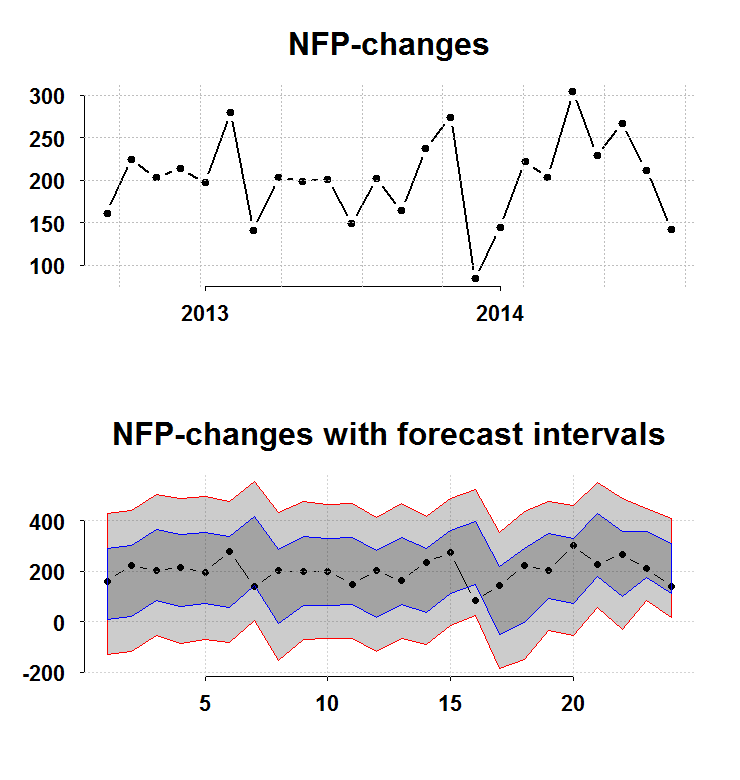
The bottom panel charts the interval you have before the number is publish (forecast intervals) from a simple AR(1) model without imposing normality. The blue and the red lines are 1 and 2 standard deviations respectively. The recent number barely scratches the bottom blue, so nothing to suggest a significant shift from a healthy 200K. On the other hand, there is some persistence:
|
1 2 3 4 5 6 7 8 9 10 11 12 13 14 |
ar.ols(na.omit(nfp)) Call: ar.ols(x = na.omit(nfp)) Coefficients: 1 2 3 4 5 6 0.2633 0.2672 0.1402 0.0841 0.1015 -0.0853 Intercept: 0.318 (5.906) Order selected 6 sigma^2 estimated as 31430 |
So, on average we can expect to trend lower.
Code for figure:
|
1 2 3 4 5 6 7 8 9 10 11 12 13 14 15 16 17 |
library(quantmod) library(Eplot) tempenv <- new.env() getSymbols("PAYEMS",src="FRED",env=tempenv) # Bring it to global env head(tempenv$PAYEMS) time <- index(tempenv$PAYEMS) nfp <- as.numeric(diff(tempenv$PAYEMS)) par(mfrow = c(2,1)) k = 24 args(plott) plott(tail(nfp,k),tail(time,k),return.to.default = F,main="NFP-changes") args(FCIplot) nfpsd <- FCIplot(nfp,k=k,rrr1="Rol",rrr2="Rol",main="NFP-changes; forecast intervals superimposed") |
Eplot (1)
Package Eplot on cran.
R vs MATLAB (Round 3)
At least for me, R by faR. MATLAB has its own way of doing things, which to be honest can probably be defended from many angles. Here are few examples for not so subtle differences between R and MATLAB:
Mom, are we bear yet?
One way to help us decide is to estimate a regime switching model for the VIX, see if the volatility crossed over to the bear regime.
Non-linear beta
If you google-finance AMZN you can see the beta is 0.93. I already wrote in the past about this illusive concept. Beta is suppose to reflect the risk of an instrument with respect for example to the market. However, you can estimate this measure in all kind of ways.
Bias vs. Consistency
Especially for undergraduate students but not just, the concepts of unbiasedness and consistency as well as the relation between these two are tough to get one’s head around. My aim here is to help with this. We start with a short explanation of the two concepts and follow with an illustration.
Bootstrap Critisim (example)
In a previous post I underlined an inherent feature of the non-parametric Bootstrap, it’s heavy reliance on the (single) realization of the data. This feature is not a bad one per se, we just need to be aware of the limitations. From comments made on the other post regarding this, I gathered that a more concrete example can help push this point across.
Detecting bubbles in real time
Recently, we hear a lot about a housing bubble forming in UK. Would be great if we would have a formal test for identifying a bubble evolving in real time, I am not familiar with any such test. However, we can still do something in order to help us gauge if what we are seeing is indeed a bubbly process, which is bound to end badly.
Bootstrap criticism
The title reads Bootstrap criticism, but in fact it should be Non-parametric bootstrap criticism. I am all in favour of Bootstrapping, but I point here to a major drawback.
My favourite statistician
We are all standing on the shoulders of giants. Bradley Efron is one such giant. With the invention of the bootstrap in 1979 and later with his very influential 2004 paper about the Least Angle Regression (and the accompanied software written in R).
R vs MATLAB – round 2
R takes it. I prefer coding in R over MATLAB. I feel R understands that I do not like to type too much. A few examples: