If you regularly read this blog then you know I am not one to jump on the “AI Bandwagon”, being quickly weary of anyone flashing the “It’s Artificial Intelligence” joker card. Don’t get me wrong, I understand it is a sexy term I, but to me it always feels a bit like a sales pitch.
If the machine does anything (artificially) intelligent it means that the model at the back is complex, and complex models need massive (massive I say) amounts of data. This is because of the infamous Curse of dimensionality.
I know it. You know it. Complex models need a lot of data. You have read this fact, even wrote it at some point. But why is it the case? “So we get a good estimate of the parameter, and a good forecast thereafter”, you reply. I accept. But.. what is it about simple models that they could suffice themselves with much less data compared to complex models? Why do I always recommend to start simple? and why the literature around shrinkage and overfitting is as prolific as it is?
Contents
Intro
Why complex models are data-hungry? I provide here a pedagogic example using bitcoin data. We look at two models. One is simple while the other is (more) complex. We use a linear model to stand for our simple model, and a 5-degree polynomial to stand for our complex model.
Start with getting the bitcoin data, prep it for fitting our models later:
|
1 2 3 4 5 6 7 8 9 10 11 |
library(quantmod) citation("quantmod") bitcoin <- getFX('BTC/USD', auto.assign = F, src='google') tt <- 150 # we use the most recent 150 days # Let's divide the data for readability x <- as.numeric(bitcoin[,1]) %>% tail(tt)/1000 degreee <- 5 # The next line creates x^2 and x^3 ply_expansion <- polym(seq(x), degree = degreee, raw = TRUE) |
This is a time series plot of the scaled data:
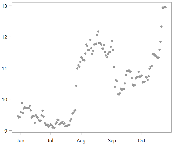
What we do next is to estimate two different models. One which is linear: lm_alot, and the other polynomial: pol_alot. Why the suffix _alot will become clear shortly. We also create an rmse function to compute the accuracy of the fitted value from our two models.
|
1 2 3 4 5 6 7 8 9 10 11 12 13 14 15 |
lm_alot <- lm(x~timee) pol_alot <- lm(x~ply_expansion) plot(x ~ timee, ylab="", pch= 19) lines(lm_alot$fit~ timee, col="darkgreen", lwd=2) lines(pol_alot$fit~ timee, col="green", lwd=2) rmse <- function(x,y){ + sqrt(mean((x - y)^2)) + } rmse(lm_alot$fit,x) [1] 0.725 rmse(pol_alot$fit,x) [1] 0.427 |
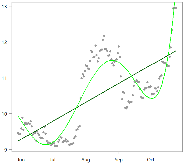
As you can see the polynomial (in light green) can of course capture the wiggly nature of this digital currency much better than our linear model.
Thought exercise
In real life we don’t see the actual underlying data-generation process. Put differently, we don’t know why the data looks the way it does (save for very particular domains like motion of stars or such). Assume we don’t see all data points, but only a fraction of them. We do this by randomly choosing 15 points from the 150 data points we actually have. We again estimate both the linear model and the polynomial one based on our new, now much smaller dataset. We replace the suffix alot with little. Both models are going to deliver different results based on our new smaller dataset, because we feed them lower number of observation to “learn” from. We start by reviewing the changes in the simple linear model, and later we see how the more complex model have changed.
|
1 2 3 4 5 6 7 8 9 10 |
set.seed(111) samp <- 15 seqq <- runif(samp, 1, tt) %>% sort %>% round lm_little <- lm(x[seqq]~timee[seqq]) plot(x ~ timee, ylab="", pch= 19) lines(lm_alot$fit~ timee, col="darkgreen", lwd=3) lines(lm_little$fit~ timee[seqq], col="darkgreen", lwd=3) points(x[seqq] ~ timee[seqq], ylab="", pch= 16, col= "black", cex=1.8) |
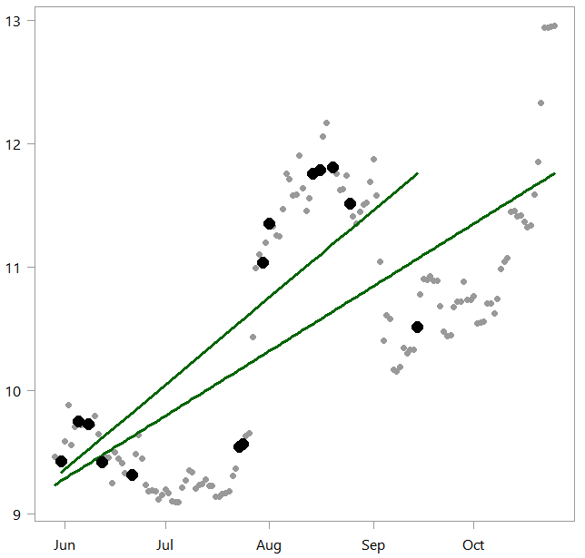
As you can see, the linear model has shifted based on the randomly sampled points (emphasized in black). It just so happened that we did not sample many points around October. So the new slope is steeper which reflects that, because there were lower bitcoin values in October which are not well-included in our randomly chosen sub-sample.
Now, how did the complex model changed?
|
1 2 3 4 5 6 7 |
pol_little <- lm(x[seqq]~ply_expansion[seqq,]) plot(x ~ timee, ylab="", pch= 19) lines(pol_alot$fit~ timee, col="green", lwd=3) lines(pol_little$fit~ timee[seqq], col="green", lwd=3) points(x[seqq] ~ timee[seqq], ylab="", pch= 16, col= "black", cex=1.8) |
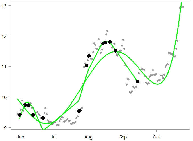 Fair enough. Looks to track the data sampled quite well around those relatively densely sampled areas (June and August).
Using our newly estimated models on the full data, a pseudo out-of-sample exercise
We now fit the data based on our newly estimated models. We also again compute the accuracy of the two models using the function rmse we wrote before.
|
1 2 3 4 5 6 7 8 9 10 11 12 |
plot(x ~ timee, ylab="", pch= 19) pred_lin <- lm_little$coef%*%t(cbind(rep(1,tt),timee)) %>% t points(pred_lin ~ timee, col="darkgreen", pch=19, cex=0.7, ty= "b") pred_pol <- pol_little$coef%*%t(cbind(rep(1,tt),ply_expansion)) %>% t points(pred_pol ~ timee, col="green", pch=19, cex=0.7, ty= "b") points(x[seqq] ~ timee[seqq], ylab="", pch= 16, col= "black", cex=1.8) rmse(pred_lin,x) [1] 0.916 rmse(pred_pol,x) [1] 14.7 |
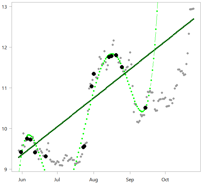
Both models are of course much worse than before. But the performance of the complex model is disastrous, with RMSE value catapulted with enormous errors. The fact that the complex model is more flexible and can wiggle with the data actually backfired in our “out-of-sample” exercise. The 15 points that we sampled did not cover well the relevant “surface” (or support in statistical language).
Complex models need massive amounts of data not because we can’t estimate them. Nowadays (yes) we can. But we get punished much more severely if the data used for estimation does not span the relevant “surface” well enough. When the data is multidimensional then spanning/covering the “surface” is hard (link to earlier curse of dimensionality post for the reason). The model-fit just drives off very fast; the more Porsche is the model the faster we drive in the wrong direction, farther away from reason. Hence the need for only gradual climb in model complexity. Simple models also suffer from the same issue. Our simple linear also drove off; out-of-sample performance is likewise much worse than our in-sample, 0.916 versus 0.725, but you don’t get into a serious accidents while riding on a donkey.

Plus 1 for simplicity, echoing William of Ockham (c. 1287–1347) who is credited with law of parsimony: “entities should not be multiplied without necessity”.
Encore – Adaptive Structural Learning of Artificial Neural Networks
I thought about this post reading the paper “AdaNet: Adaptive Structural Learning of Artificial Neural Networks” which, I think, could have been more popular with more friendly math notations. Given the lack of theoretical underpinnings for deep learning models, there is little guidance on specifying model architecture. I suspect the issue will remain open for years to come. Think about what information criteria is doing: penalizing you for adding parameters without “enough” compensating accuracy raise. The paper suggests something similar. Start simple, add complexity, check performance and stop if accuracy raise is not enough for the added complexity. It’s not an easy read. Unlike information criteria like AIC say, we can’t simply count how complex is the model the way we can count the number of regressors for example. The authors negotiate around it by suggesting to use a function-complexity measure. Interesting, not for everyone but for you yes.
References


2 comments on “Why complex models are data-hungry?”