What is tail dependence really? Say the market had a red day and saw a drawdown which belongs with the 5% worst days (from now on simply call it a drawdown):
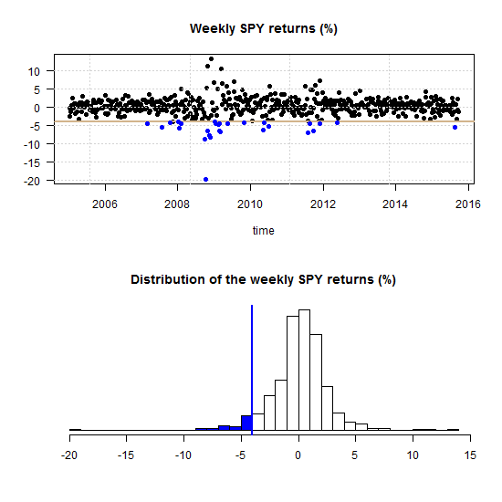
One can ask what is now, given that the market is in the blue region, the probability of a a drawdown in a specific stock?
Category: Finance and Trading
Multivariate volatility forecasting (4), factor models
To be instructive, I always use very few tickers to describe how a method works (and this tutorial is no different). Most of the time is spent on methods that we can easily scale up. Even if exemplified using only say 3 tickers, a more realistic 100 or 500 is not an obstacle. But, is it really necessary to model the volatility of each ticker individually? No.
If we want to forecast the covariance matrix of all components in the Russell 2000 index we don’t leave much on the table if we model only a few underlying factors, much less than 2000.
Volatility factor models are one of those rare cases where the appeal is both theoretical and empirical. The idea is to create a few principal components and, under the reasonable assumption that they drive the bulk of comovement in the data, model those few components only.
Multivariate volatility forecasting (3), Exponentially weighted model
Broadly speaking, complex models can achieve great predictive accuracy. Nonetheless, a winner in a kaggle competition is required only to attach a code for the replication of the winning result. She is not required to teach anyone the built-in elements of his model which gives the specific edge over other competitors. In a corporation settings your manager and his manager and so forth MUST feel comfortable with the underlying model. Mumbling something like “This artificial-neural-network is obtained by using a grid search over a range of parameters and connection weights where the architecture itself is fixed beforehand…”, forget it!
Multivariate volatility forecasting, part 2 – equicorrelation
Last time we showed how to estimate a CCC and DCC volatility model. Here I describe an advancement labored by Engle and Kelly (2012) bearing the name: Dynamic equicorrelation. The idea is nice and the paper is well written.
Departing where the previous post ended, once we have (say) the DCC estimates, instead of letting the variance-covariance matrix be, we force some structure by way of averaging correlation across assets. Generally speaking, correlation estimates are greasy even without any breaks in dynamics, so I think forcing some structure is for the better.
Correlation and correlation structure (1); quantile regression
Given a constant speed, time and distance are fully correlated. Provide me with the one, and I’ll give you the other. When two variables have nothing to do with each other, we say that they are not correlated.
You wish that would be the end of it. But it is not so. As it is, things are perilously more complicated. By far the most familiar correlation concept is the Pearson’s correlation. Pearson’s correlation coefficient checks for linear dependence. Because of it, we say it is a parametric measure. It can return an actual zero even when the two variables are fully dependent on each other (link to cool chart).
Multivariate volatility forecasting (1)
Introduction
When hopping from univariate volatility forecasts to multivariate volatility forecast, we need to understand that now we have to forecast not only the univariate volatility element, which we already know how to do, but also the covariance elements, which we do not know how to do, yet. Say you have two series, then this covariance element is the off-diagonal of the 2 by 2 variance-covariance matrix. The precise term we should use is “variance-covariance matrix”, since the matrix consists of the variance elements on the diagonal and the covariance elements on the off-diagonal. But since it is very tiring to read\write “variance-covariance matrix”, it is commonly referred to as the covariance matrix, or sometimes less formally as var-covar matrix.
Energy idiosyncratic volatility
Recently, volatility has been on the up. Generally, we associate rising volatility with a bear regime, but we also know there is a percolating oil shock. Is the volatility we see in the stock market broad-based, or is it the effect brought about by sharp the drop in oil prices (so related to the energy sector)? I propose here a practical way to take a closer look at it.
Fed Fund Rate futures curve and what they tell us
“The Fed is certainly moving forward with plans to normalize interest rates.” We keep on hearing that, we believed it in the past and we believe it now. We believe that the Fed believes and that, in fact, this means something.
Should we become more suspicious and less trusting given history? Let’s take a look.
Linking backtesting with multiple testing
The other day, Harvey Campbell from Duke University gave a talk where I work. The talk- bearing the exciting name “Backtesting” was based on a paper by the same name.
The authors tackle the important problem of data-snooping; we need to account for the fact that we conducted many trials until we found a strategy (or a variable) that ‘works’. Accessible explanations can be found here and here. In this day and age, the ‘story’ behind what you are doing is more important than ever, given the things you can do using your desktop/laptop.
Mom, are we bear yet? (2)
5 weeks ago we took a look at the rising volatility in the (US) equity markets via a time-series threshold model for the VIX. The estimate suggested we are crossing (or crossed) to the more volatile regime. Here, taking somewhat different Hidden Markov Model (HMM) approach we gather more corroboration (few online references at the bottom if you are not familiar with HMM models. The word hidden since the state is ‘invisible’).
On the nonfarm payroll number
The total nonfarm payroll accounts for approximately 80% of the workers who produce the GDP of the United States. Despite the widely acknowledged fact that the Nonfarm payroll is highly volatile and is heavily revised, it is still driving both bonds and equity market moves before- and after it is published. The recent number came at a weak 142K compared with around 200K average over the past 12M. What we wish we would know now, but will only know later, is whether this number is a start of a weaker expansion in the workforce, or not.
Despite the fact that it is definitely on the weak side (as you can see in the top panel of the figure), it is nothing unusual (as you can see in the bottom panel of the figure).
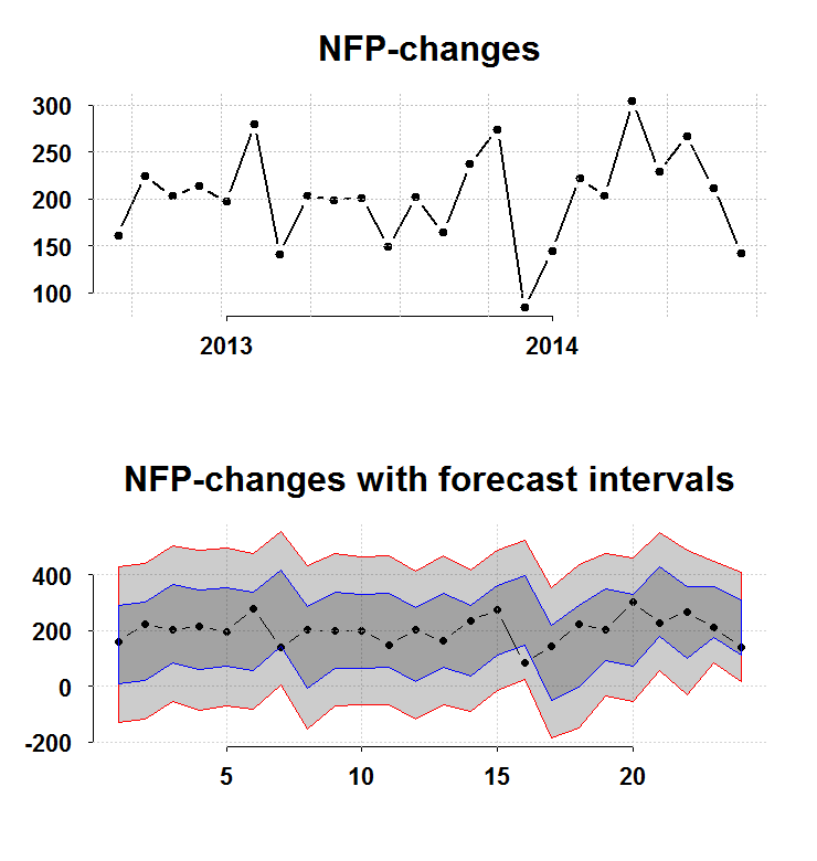
The bottom panel charts the interval you have before the number is publish (forecast intervals) from a simple AR(1) model without imposing normality. The blue and the red lines are 1 and 2 standard deviations respectively. The recent number barely scratches the bottom blue, so nothing to suggest a significant shift from a healthy 200K. On the other hand, there is some persistence:
ar.ols(na.omit(nfp))

Call:
ar.ols(x = na.omit(nfp))

Coefficients:
      1        2        3        4        5        6
 0.2633   0.2672   0.1402   0.0841   0.1015  -0.0853

Intercept: 0.318 (5.906)

Order selected 6  sigma^2 estimated as  31430
So, on average we can expect to trend lower.
Code for figure:
library(quantmod)
library(Eplot)

tempenv <- new.env()
getSymbols("PAYEMS",src="FRED",env=tempenv)
# Bring it to global env
head(tempenv$PAYEMS)
time <- index(tempenv$PAYEMS)
nfp <- as.numeric(diff(tempenv$PAYEMS))
par(mfrow = c(2,1))
k = 24
args(plott)
plott(tail(nfp,k),tail(time,k),return.to.default = F,main="NFP-changes")
args(FCIplot)
nfpsd <- FCIplot(nfp,k=k,rrr1="Rol",rrr2="Rol",main="NFP-changes; forecast intervals superimposed")
Mom, are we bear yet?
One way to help us decide is to estimate a regime switching model for the VIX, see if the volatility crossed over to the bear regime.
Non-linear beta
If you google-finance AMZN you can see the beta is 0.93. I already wrote in the past about this illusive concept. Beta is suppose to reflect the risk of an instrument with respect for example to the market. However, you can estimate this measure in all kind of ways.
Detecting bubbles in real time
Recently, we hear a lot about a housing bubble forming in UK. Would be great if we would have a formal test for identifying a bubble evolving in real time, I am not familiar with any such test. However, we can still do something in order to help us gauge if what we are seeing is indeed a bubbly process, which is bound to end badly.
Bootstrap criticism
The title reads Bootstrap criticism, but in fact it should be Non-parametric bootstrap criticism. I am all in favour of Bootstrapping, but I point here to a major drawback.