To be instructive, I always use very few tickers to describe how a method works (and this tutorial is no different). Most of the time is spent on methods that we can easily scale up. Even if exemplified using only say 3 tickers, a more realistic 100 or 500 is not an obstacle. But, is it really necessary to model the volatility of each ticker individually? No.
If we want to forecast the covariance matrix of all components in the Russell 2000 index we don’t leave much on the table if we model only a few underlying factors, much less than 2000.
Volatility factor models are one of those rare cases where the appeal is both theoretical and empirical. The idea is to create a few principal components and, under the reasonable assumption that they drive the bulk of comovement in the data, model those few components only.
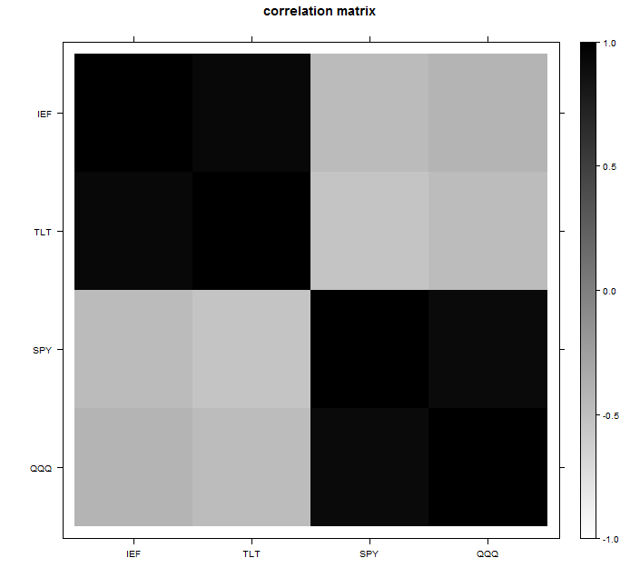
For the example we can use four tickers: ‘IEF’,’TLT’, ‘SPY’, ‘QQQ’. The first two track the short and longer term bond returns, and the last two track some equity indexes. You can look at the correlation matrix and guess two factors are enough for this data:
library(quantmod)
k <- 5 # how many years back?
end<- format(Sys.Date(),"%Y-%m-%d")
start<-format(Sys.Date() - (k*365),"%Y-%m-%d")
symetf = c('IEF','TLT', 'SPY', 'QQQ')
l <- length(symetf)
dat0 = getSymbols(symetf[1], src="yahoo", from=start, to=end, auto.assign = F, warnings = FALSE,symbol.lookup = F)
n = NROW(dat0)
dat = array(dim = c(n,NCOL(dat0),l)) ; ret = matrix(nrow = n, ncol = l)
for (i in 1:l){
  dat0 = getSymbols(symetf[i], src="yahoo", from=start, to=end, auto.assign = F,
                    warnings = FALSE,symbol.lookup = F)
  dat[1:n,,i] = dat0
  ret[2:n,i] = 100*(dat[2:n,4,i]/dat[1:(n-1),4,i] - 1) # returns, close to close, percentage
}
ret <- na.omit(ret)# Remove the first observation
time <- as.Date(substr(index(dat0),1,10))[-1]
TT <- NROW(ret)
#-----------------------------------
pc0 <- prcomp(ret, scale=T)
par(mfrow = c(2,1))
plot(pc0, las = 1, main = "Variance of the principal component")
barplot(summary(pc0)$import[2,], las = 1, main = "Proportion of variance explained")
You see the two blocks? you can ask the software to construct principal components and see how much is explained by each factor. The feeling that only two factors are needed here is then confirmed by looking at the percentage of variance explained:
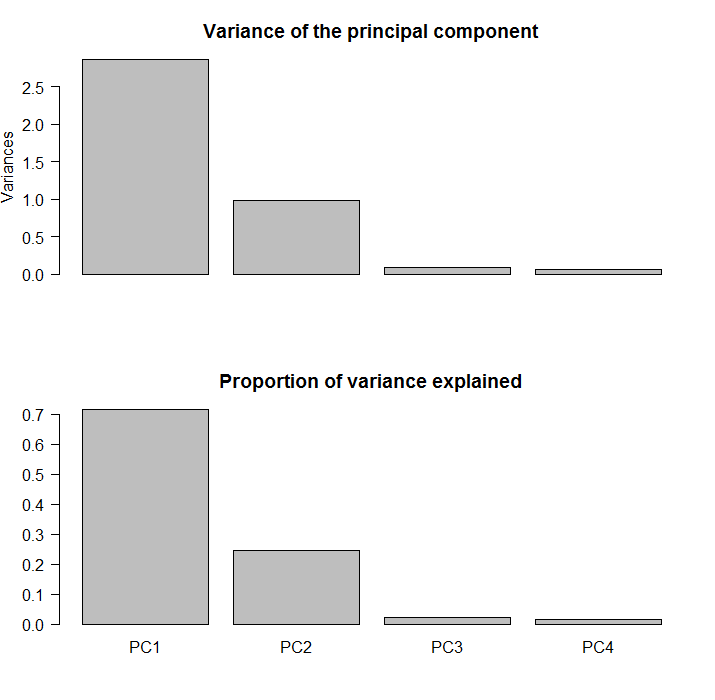
The first two component explain about 90% of the comovement in the data.
Now, we can use something which bears the antagonistic name matrix spectral decomposition. We decompose the covariance matrix  into a series of summable matrices:
(1) 
where the eigenvalues and the corresponding eigenvectors are organized from the largest (which is first) to the smallest (which is last). The bold face is to clarify those are vectors, as oppose to scalars. I have no intuitive explanation for why it is called spectral (why not “sweet matrix decomposition”?). Equation (1) is the principal component estimator for the covariance matrix. We can use singular value decomposition to compute this. We have a maximum of 4 factors, the same as the number of tickers. If our aim is the correlation matrix we can standardize the data. We don’t have to sum up all 4 matrices, we can stop after only two, essentially using only two factors. I change now notation from to  underscoring that is based on all factors.
(2) 
where
(3) ![\begin{equation*} \Gamma = [eigenvalue_1 \times \mathbf{eigenvector_i}, ... ,eigenvalue_k \times \mathbf{eigenvector_k} ], \end{equation*}](https://eranraviv.com/wp-content/ql-cache/quicklatex.com-af665dff967feb9fa09439ab327ed91d_l3.svg "Rendered by QuickLaTeX.com")
but now  so we don’t use all possible factors, and the rest of the “comovement” enters the freshly introduced matrix
  .
.
Think of this matrix as the garbage can for the unexplained comovement:
(4) 
This allow us the estimate based on a factor volatility model in equation (2). The ordering:
- standardize
- Create single value decomposition
- Decide how many factors to use and calculate
 based on (3)
 - Calculate the residual matrix based on (4)
- Get the estimate in equation (2)
The code, for a better understanding. Using all of them we simply get the sample correlation matrix:
sret <- scale(ret) # We standardize because we want the correlation, not the covariance
xpx <- t(sret)%*%sret/(NROW(ret)-1)
eigval = eigen(xpx, symmetric=T)
rescaled_loadingsl <- NULL
for (i in 1:l){
  rescaled_loadings0 <- sqrt(eigval$values[i]) * (eigval$vectors[,i])
  rescaled_loadingsl <- cbind(rescaled_loadingsl, rescaled_loadings0)
}
colnames(rescaled_loadingsl) <- c(paste("scaled_load",1:l,sep=""))
Sl <- rescaled_loadingsl%*%t(rescaled_loadingsl)
> Sl
       [,1]   [,2]   [,3]   [,4]
[1,]  1.000  0.915 -0.471 -0.413
[2,]  0.915  1.000 -0.536 -0.466
[3,] -0.471 -0.536  1.000  0.930
[4,] -0.413 -0.466  0.930  1.000
> cor(ret)
       [,1]   [,2]   [,3]   [,4]
[1,]  1.000  0.915 -0.471 -0.413
[2,]  0.915  1.000 -0.536 -0.466
[3,] -0.471 -0.536  1.000  0.930
[4,] -0.413 -0.466  0.930  1.000
>
Here we take the trouble to construct our own PC’s, without using the build-in function, but we don’t have to really. We do it to get better understanding of what is going on, but you can use the easy built-in prcomp function to get the same:
pc <- sret%*%eigval$vectors # eigval$vectors are the factor loadings!
pc0 <- prcomp(ret, scale=T)
> head(pc0$x, 2)
        PC1    PC2    PC3    PC4
[1,] -0.776  0.786 0.1799  0.365
[2,] -1.436 -1.149 0.0452 -0.024
> head(pc, 2)
       [,1]   [,2]    [,3]   [,4]
[1,] -0.776 -0.786 -0.1799 -0.365
[2,] -1.436  1.149 -0.0452  0.024
> tail(pc0$x, 2)
           PC1   PC2   PC3   PC4
[1256,] -2.174 0.796 0.255 0.130
[1257,] -0.494 0.276 0.133 0.154
> tail(pc, 2)
          [,1]   [,2]   [,3]   [,4]
[1256,] -2.174 -0.796 -0.255 -0.130
[1257,] -0.494 -0.276 -0.133 -0.154
#-----------------------------
> apply(pc,2,sd)
[1] 1.693 0.992 0.293 0.254
> sqrt(eigval$values[])
[1] 1.693 0.992 0.293 0.254
#-----------------------------
# plot(pc[,1]~pc0$x[,1]) # If you want..
Let’s now construct an estimate of the correlation matrix based only on two factors:
k <- 2 # From previous section we know 2 are enough
rescaled_loadings <- NULL
for (i in 1:k){
rescaled_loadings0 <- sqrt(eigval$values[i]) * (eigval$vectors[,i])
rescaled_loadings <- cbind(rescaled_loadings, rescaled_loadings0)
}
Sigma <- rescaled_loadings%*%t(rescaled_loadings)
colnames(rescaled_loadings) <- c(paste("scaled_load",1:k,sep=""))
> Sigma
       [,1]   [,2]   [,3]   [,4]
[1,]  0.960  0.956 -0.474 -0.406
[2,]  0.956  0.957 -0.535 -0.470
[3,] -0.474 -0.535  0.965  0.963
[4,] -0.406 -0.470  0.963  0.967
> cor(ret)
       [,1]   [,2]   [,3]   [,4]
[1,]  1.000  0.915 -0.471 -0.413
[2,]  0.915  1.000 -0.536 -0.466
[3,] -0.471 -0.536  1.000  0.930
[4,] -0.413 -0.466  0.930  1.000
Ha, Sigma now does not look like a correlation matrix. We need to add the Omega from equation (4):
omg_eps <- diag(diag(Sl - (rescaled_loadings%*%t(rescaled_loadings))))
# the "diag(diag(" is a bit clumsy, but it does follow the math
sig_hat <- Sigma + omg_eps
cat("compare" , "\n"); cor(ret);cat("with" ,"\n")
compare
       [,1]   [,2]   [,3]   [,4]
[1,]  1.000  0.915 -0.471 -0.413
[2,]  0.915  1.000 -0.536 -0.466
[3,] -0.471 -0.536  1.000  0.930
[4,] -0.413 -0.466  0.930  1.000
with
       [,1]   [,2]   [,3]   [,4]
[1,]  1.000  0.956 -0.474 -0.406
[2,]  0.956  1.000 -0.535 -0.470
[3,] -0.474 -0.535  1.000  0.963
[4,] -0.406 -0.470  0.963  1.000
So, only slightly different. Again, for 4 tickers this is pretty useless staff. But for a well diversified 2000 names portfolio, this method can serve us well.


