Intraday volatility measures

In the last few decades there has been tremendous progress in the realm of volatility estimation. A major step is the additional use of intraday price path. It has been shown that estimates which consider intraday information are more accurate. Which is to say they converge faster to the real unobserved value of the true volatility.

It makes perfect sense. The usual proxy you’ve heard about, $\varepsilon^2$ only uses 2 information points, close-to-close, the following measures use much more information. They are termed range based, as they examine the range at some interval (one minute in my example) and sum them up to get the desired daily estimate. So, more information since they consider the full path in each day.

SPY - Daily Return Path - most recent year — SPY – Daily Return Path – most recent year

I present three estimators. They have solid theory to back them up, however, as with any step forward, we face new tough decisions. I refer specifically to the number of intervals, (here one minute intervals so 390). From my experience it is quite important and it has to do with market micro-structure and the bid-ask spreads, in the references you can find a related paper. Let’s move on to the R code:

Here are three options, in all formulas $h_i, l_i, cl_i, o_i$ are high, low, close and open prices for interval i respectively.

Parkinson (1980):

(1) $\begin{equation*} \sigma = \sqrt{\frac{1}{4Nln2}\sum_{i = 1}^N(ln\frac{h_i}{l_i})^2} \end{equation*}$


# Parkinson Volatility Estimator
Park = function(x){   
	# x is an array of prices with dimension:
	# (num.intervals.each.day)*( (5 or 6), "open", "high" etc)*(number.days) 
	n <- dim(x)[1] # number of intervals each day. 
	l <- dim(x)[3] # number of days, most recent year in my this post
	pa = NULL
	
	for (i in 1:l) {
		log.hi.lo <- log( x[1:n,2,i]/x[1:n,3,i] ) 
		pa[i] =  sum( log.hi.lo^2 )  / (4*n*log(2))
	}
	return(pa)
}

# Parkinson Volatility Estimator

Park = function(x){

# x is an array of prices with dimension:

# (num.intervals.each.day)*( (5 or 6), "open", "high" etc)*(number.days)

n <- dim(x)[1] # number of intervals each day.

l <- dim(x)[3] # number of days, most recent year in my this post

pa = NULL

for (i in 1:l) {

log.hi.lo <- log( x[1:n,2,i]/x[1:n,3,i] )

pa[i] = sum( log.hi.lo^2 ) / (4*n*log(2))

}

return(pa)

}

Garman Klass (1980):

(2) $\begin{equation*} \sigma = \sqrt{\frac{1}{N}\sum_{i = 1}^N\frac{1}{2}(ln\frac{h_i}{l_i})^2 - \frac{1}{N}\sum_{i = 1}^N(2ln2-1)(ln\frac{c_i}{c_{i-1}})^2} \end{equation*}$


# Garman-Klass Volatility Estimator
GarmanKlass = function(x){   
	# x is an array of prices with dimension:
	# (num.intervals.each.day)*( (5 or 6), "open", "high" etc)*(number.days) 
	n <- dim(x)[1] # number of intervals each day. 
 l <- dim(x)[3] # number of days 
gk = NULL
	for (i in 1:l) {
	log.hi.lo <- log( x[1:n,2,i]/x[1:n,3,i] )
	log.cl.to.cl <- log( x[2:n,4,i]/x[1:(n-1),4,i] )
		gk[i] = ( sum(.5*log.hi.lo^2) - sum( (2*log(2) - 1)*(log.cl.to.cl^2) ) ) /n
	}
	return(gk)
}

# Garman-Klass Volatility Estimator

GarmanKlass = function(x){

# x is an array of prices with dimension:

# (num.intervals.each.day)*( (5 or 6), "open", "high" etc)*(number.days)

n <- dim(x)[1] # number of intervals each day.

l <- dim(x)[3] # number of days

gk = NULL

for (i in 1:l) {

log.hi.lo <- log( x[1:n,2,i]/x[1:n,3,i] )

log.cl.to.cl <- log( x[2:n,4,i]/x[1:(n-1),4,i] )

gk[i] = ( sum(.5*log.hi.lo^2) - sum( (2*log(2) - 1)*(log.cl.to.cl^2) ) ) /n

}

return(gk)

}

Rogers and satchell (1991):

(3) $\begin{equation*} \sigma = \sqrt{\frac{1}{N}\sum_{i = 1}^N(ln\frac{h_i}{l_i})(ln\frac{h_i}{o_i}) + (ln\frac{l_i}{c_{i}}) (ln\frac{l_i}{o_{i}})} \end{equation*}$


# Roger and Satchell Volatility Estimator
RogerSatchell = function(x){   
	# x is an array of prices with dimension:
	# (num.intervals.each.day)*( (5 or 6), "open", "high" etc)*(number.days) 
	n <- dim(x)[1] # number of intervals each day. 
	l <- dim(x)[3] # number of days 
	rs = NULL

	for (i in 1:l) {
		log.hi.cl <- log( x[1:n,2,i]/x[1:n,4,i] ) 
		log.hi.op <- log( x[1:n,2,i]/x[1:n,1,i] )
		log.lo.cl <- log( x[1:n,3,i]/x[1:n,4,i] ) 
		log.lo.op <- log( x[1:n,3,i]/x[1:n,1,i] )
	
		rs[i] =  sum( log.hi.cl*log.hi.op + log.lo.cl*log.lo.op )  /n
	}
	return(rs)
}

# Roger and Satchell Volatility Estimator

RogerSatchell = function(x){

# x is an array of prices with dimension:

# (num.intervals.each.day)*( (5 or 6), "open", "high" etc)*(number.days)

n <- dim(x)[1] # number of intervals each day.

l <- dim(x)[3] # number of days

rs = NULL

for (i in 1:l) {

log.hi.cl <- log( x[1:n,2,i]/x[1:n,4,i] )

log.hi.op <- log( x[1:n,2,i]/x[1:n,1,i] )

log.lo.cl <- log( x[1:n,3,i]/x[1:n,4,i] )

log.lo.op <- log( x[1:n,3,i]/x[1:n,1,i] )

rs[i] = sum( log.hi.cl*log.hi.op + log.lo.cl*log.lo.op ) /n

}

return(rs)

}

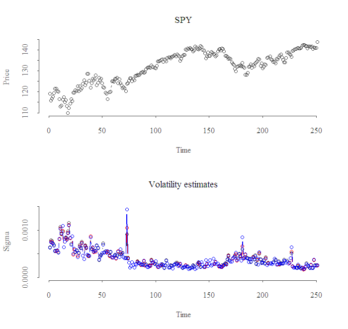
The result for the most recent year is:

As you can see the correlation between the estimates is very high, which is in some sense comforting since it assures code validity, yet it also means that it does not really matter with which one you choose to go.


cor(cbind(sqrt(v1),sqrt(v2),sqrt(v3)), use = "complete.obs")
      [,1]  [,2]  [,3]
[1,] 1.000 0.989 0.997
[2,] 0.989 1.000 0.977
[3,] 0.997 0.977 1.000