Smoothed Bootstrap

This post discusses the need for smoothed version of the statistical bootstrap. I start with a negative result of the standard bootstrap, and introduce smoothing as a practical, and necessary improvement.

Suppose you have 100 unique values and you draw a new sample of 100 observations with replacement. How many unique values would you expect to see in this new sample?
➡️
On average, fewer than 70 of the original values would appear. Unfortunately, you are deprived of using more than 30% of your data, and that is hard to remedy.

Why does ~30% of your data end up being left out of each sample?

The Probability of an Observation Being “Left Behind”

For a sample of 100 unique values, the probability of a single observation being included in the bootstrap sample is $\frac{1}{100}$ . So the probability of being excluded is $\frac{99}{100} = 1 - \frac{1}{100}$ . For the number of your independent draws (100 in our example):

$\left(1 - \frac{1}{100}\right)^{100} \approx 0.366,$

(or 36.6%). And more generally, as the sample size $N$ grows this formula converges to $1 - \frac{1}{e} \approx 63.21\%$ . Therefore, your bootstrap sample is expected to capture only 63 unique values, meaning the remaining 37 are duplicates (not unique).

Practical implications

Look at the below Rython code as a thought exercise. I compare how often Shapiro-Wilk normality test rejects the null hypothesis (i.e., concludes the data is not normal) in two scenarios: for the true distribution (simulated from normal), and for a boostrap sample from the original sample (which is of course coming from normal distribution). We know that the original data is normally distributed because that is how it was simulated, and so the p-values are indeed uniformly distributed, with a low percentage of rejection (around 6-7%) as expected. But, for the bootstrap sample, even though it should approximate the underlying true distribution, the rejection rate (incorrectly concluding that the data is not normally distributed) is extremely high at around 45%. See also the figure directly after the code for the distribution of the p-values.

m <-  100
n_sim <- 100
p_values_orig <- p_values_boot <- NULL
for (i in 1:n_sim){
x <- rnorm(m)
p_values_orig[i] <- shapiro.test(x)$p.value
y <- sample(x, size= m, replace= T)
p_values_boot[i] <- shapiro.test(y)$p.value
}
1 - sum((p_values_boot>0.05))/n_sim
[1] 0.44
1 - sum((p_values_orig>0.05))/n_sim
[1] 0.07

import numpy as np
from scipy.stats import shapiro
m = 100
n_sim = 100
p_values_orig = np.zeros(n_sim)
p_values_boot = np.zeros(n_sim)
for i in range(n_sim):
    x = np.random.randn(m)
    p_values_orig[i] = shapiro(x).pvalue
    y = np.random.choice(x, size=m, replace=True)
    p_values_boot[i] = shapiro(y).pvalue
print(1 - np.sum(p_values_orig > 0.05) / n_sim)
0.060
print(1 - np.sum(p_values_boot > 0.05) / n_sim)
0.470

Shapiro-Wilk p-values (n=100): Original Normal Samples vs Bootstrap Samples

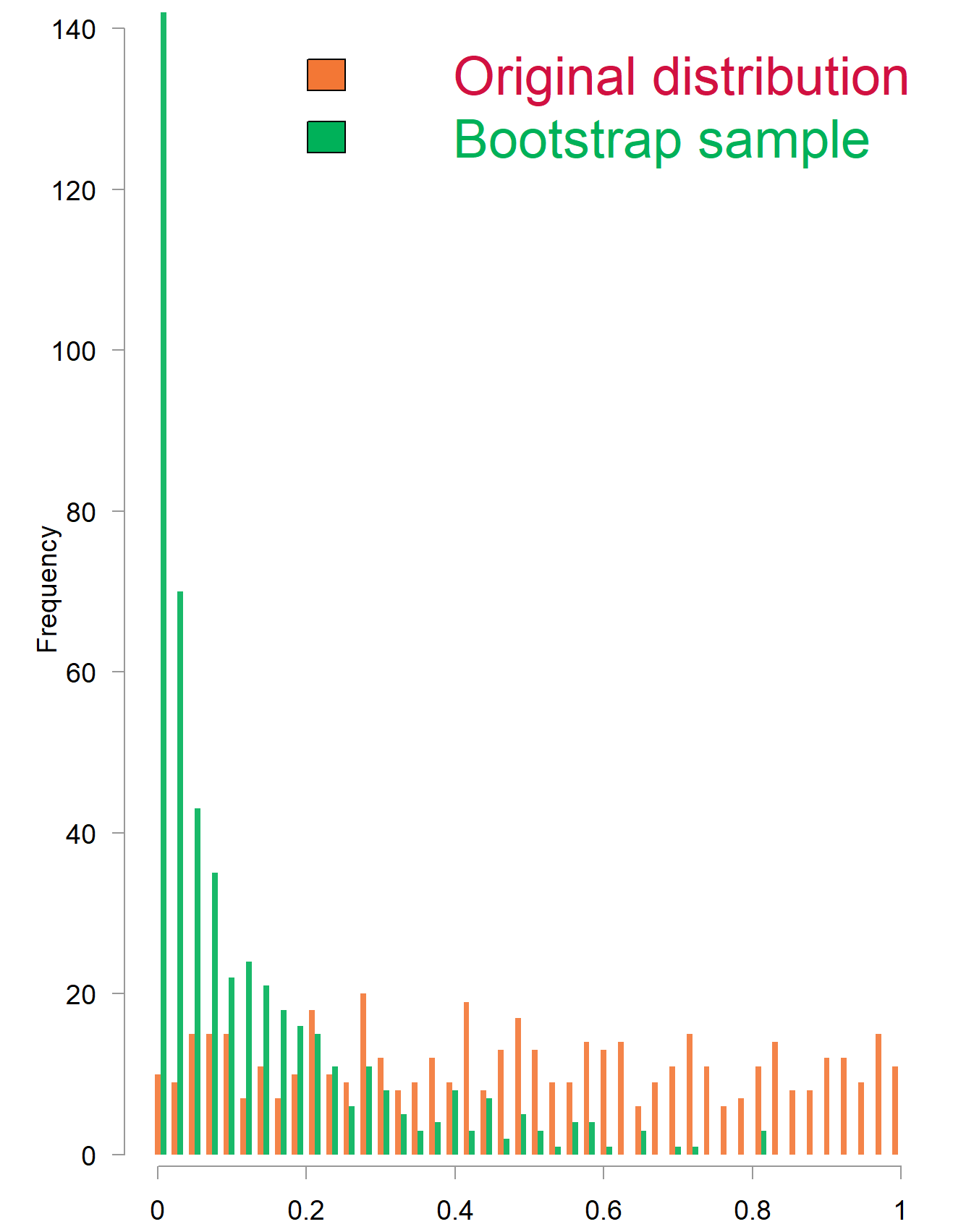
Figure 1. The green distribution highlights that the test often wrongly rejects normality on bootstrap samples (many low p-values), whereas the orange distribution reflects the correct behavior for actual normal data.

Given what we know about the powers of the bootstrap, you are undoubtedly scratching your head in bewilderment. If the empirical distribution

$\hat{F}_n \xrightarrow{a.s.} F,$

and by construction, a bootstrap sample drawn from $\hat{F}_n$ converges back to $\hat{F}_n$ as the number of bootstrap draws grows. Composing the two, one is entitled to expect the bootstrap sample to converges to $F$ . It’s simply the logical sequence: $\hat{F}_n^* \xrightarrow{a.s.} \hat{F}_n \quad \text{as } B \to \infty, \text{and } \hat{F}_n \xrightarrow{a.s.} F \quad \text{as } n \to \infty$ . And indeed, for most functionals that logic works perfectly. But not for all functionals (see another example here).

What seems to be the problem officer?

In the example above the functional is the density, which is continuous. naïve bootstrap forces a continuous distribution to collapse into a jagged, discrete grid, full of repeating duplicates as explained above – this is the root cause of the failure we observe.

To mitigate this problem, we should doctor the bootstrap with some healthy smoothing.

Smoothed Bootstrap

For a functional $a(F)$ , the smoothed bootstrap estimate is:

$\hat{a}_h = a(\hat{F}_h),$

so not $a(\hat{F}_n)$ but $a(\hat{F}_h)$ . In practice you sample observations as usual and inject some noise to them: $X_i^* = X_i + h \varepsilon$ with $\varepsilon$ from some predefined or estimated distribution, and $h$ is the variability of the noise (i.e., a larger variance results in a smoother density for the sample). Or, equivalently, you can estimate the density of the original sample with bandwidth $h$ playing the same role of controlling the jaggedness. Using this solution will not completely fix the discrete nature of the bootstrap; but it will substantially lessen the problem. I give the math of how to implement a simple smooth bootstrap and the code follows exactly.

You estimate the density of the original sample $\hat{f}$ and use the empirical CDF based on that density estimate:

$\hat{F}(x) = \frac{\displaystyle\sum \hat{f}(x_i) \cdot \mathbb{I}(x_i \leq x)}{\displaystyle\sum \hat{f}(x_i)}$

Then you draw smoothed samples as:

$y^*_i = \hat{F}^{-1}(U_i), \quad U_i \sim \mathcal{U}(0,1)$

Example implementation code shows that if you do that the rejection rate drops from ~45% to around 15%, bringing it closer to our ideal 5% target.

 p_values_smooth_boot <- NULL
 for (i in 1:n_sim){
 x <- rnorm(m)
 dens <- density(x)
 cdf <- cumsum(dens$y) / sum(dens$y)
 inverse_cdf <- approxfun(cdf, dens$x)
 y_smoothed <- inverse_cdf(runif(m))
 p_values_smooth_boot[i] <- shapiro.test(y_smoothed)$p.value
 }
1 - sum((p_values_smooth_boot>0.05))/n_sim
[1] 0.15

A final word. We can do better for functionals that require smoothness with respect to the data, but some risk involved. In particular the smooth bootstrap is quite sensitive to the choice of bandwidth as shown in a referenced paper below. And of course, obtaining an optimal smoothing estimate requires additional effort, and introduce additional estimation noise. But, the benefits justify the effort in many scenarios. Very many important statistical quantities are not smooth with respect to the data; so it’s good to keep the smoothed bootstrap in your back pocket for when you need it.