Density estimation belongs with the literature of non-parametric statistics. Using simple bootstrapping techniques we can obtain confidence intervals (CI) for the whole density curve. Here is a quick and easy way to obtain CI’s for different risk measures (VaR, expected shortfall) and using what follows, you can answer all kind of relevant questions.
Tag: Econometric
On Central Moments
Sometimes I read academic literature, and often times those papers contain some proofs. I usually gloss over some innocent-looking assumptions on moments’ existence, invariably popping before derivations of theorems or lemmas. Here is one among countless examples, actually taken from Making and Evaluating Point Forecasts:
Modeling Tail Behavior with EVT
Extreme Value Theory (EVT) and Heavy tails
Extreme Value Theory (EVT) is busy with understanding the behavior of the distribution, in the extremes. The extreme determine the average, not the reverse. If you understand the extreme, the average follows. But, getting the extreme right is extremely difficult. By construction, you have very few data points. By way of contradiction, if you have many data points then it is not the extreme you are dealing with.
Good coding practices – part 2
Introduction
In part 1 of Good coding practices we considered how best to code for someone else, may it be a colleague who is coming from Excel environment and is unfamiliar with scripting, a collaborator, a client or the future-you, the you few months from now. In this second part, I give some of my thoughts on how best to write functions, the do’s and dont’s.
Forecast averaging example
Especially in economics/econometrics, modellers do not believe their models reflect reality as it is. No, the yield curve does NOT follow a three factor Nelson-Siegel model, the relation between a stock and its underlying factors is NOT linear, and volatility does NOT follow a Garch(1,1) process, nor Garch(?,?) for that matter. We simply look at the world, and try to find an apt description of what we see.
Measurement error bias
What is measurement error bias?
Errors-in-variables, or measurement error situation happens when your right hand side variable(s); your $x$ in a $y_t = \alpha + \beta x_t + \varepsilon_t$ model is measured with error. If $x$ represents the price of a liquid stock, then it is accurately measured because the trading is so frequent. But if $x$ is a volatility, well, it is not accurately measured. We simply don’t yet have the power to tame this variable variable.
Unlike the price itself, volatility estimates change with our choice of measurement method. Since no model is a perfect depiction of reality, we have a measurement error problem on our hands.
Ignoring measurement errors leads to biased estimates and, good God, inconsistent estimates.
The case for Regime-Switching GARCH
GARCH models are very responsive in the sense that they allow the fit of the model to adjust rather quickly with incoming observations. However, this adjustment depends on the parameters of the model, and those may not be constant. Parameters’ estimation of a GARCH process is not as quick as those of say, simple regression, especially for a multivariate case. Because of that, I think, the literature on time-varying GARCH is not yet at its full speed. This post makes the point that there is a need for such a class of models. I demonstrate this by looking at the parameters of Threshold-GARCH model (aka GJR GARCH), before and after the 2008 crisis. In addition, you can learn how to make inference on GARCH parameters without relying on asymptotic normality, i.e. using bootstrap.
Curse of dimensionality part 2: forecast combinations
In a previous post we discussed the term ‘curse of dimensionality’ and showed how it manifests itself, in practice. Here we give another such example.
Linear regression assumes nothing about your data
We often see statements like “linear regression makes the assumption that the data is normally distributed”, “Data has no or little multicollinearity”, or other such blunders (you know who you are..).
Let’s set the whole thing straight.
Linear regression assumes nothing about your data
It has to be said. Linear regression does not even assume linearity for that matter, I argue. It is simply an estimator, a function. We don’t need to ask anything from a function.
Consider that linear regression has an additional somewhat esoteric, geometric interpretation. When we perform a linear regression you simply find the best possible, closest possible, linear projection we can. A linear combination in your X space that is as close as possible in a Euclidean sense (squared distance) to some other vector y.
That is IT! a simple geometric relation. No assumptions needed whatsoever.
You don’t ask anything from the average when you use it as an estimate for the mean do you? So why do that when you use regression? We only need to ask more if we do something more.
Curse of dimensionality part 1: Value at Risk
The term ‘curse of dimensionality’ is now standard in advanced statistical courses, and refers to the disproportional increase in data which is needed to allow only slightly more complex models. This is true in high-dimensional settings. Here is an illustration of the ‘Curse of dimensionality’ in action.
Present-day great statistical discoveries
Some time during the 18th century the biologist and geologist Louis Agassiz said: “Every great scientific truth goes through three stages. First, people say it conflicts with the Bible. Next they say it has been discovered before. Lastly they say they always believed it”. Nowadays I am not sure about the Bible but yeah, it happens.
I express here my long-standing and long-lasting admiration for the following triplet of present-day great discoveries. The authors of all three papers had initially struggled to advance their ideas, which echos the quote above. Here they are, in no particular order.
Multivariate volatility forecasting (5), Orthogonal GARCH
In multivariate volatility forecasting (4), we saw how to create a covariance matrix which is driven by few principal components, rather than a complete set of tickers. The advantages of using such factor volatility models are plentiful.
Correlation and correlation structure (3), estimate tail dependence using regression
What is tail dependence really? Say the market had a red day and saw a drawdown which belongs with the 5% worst days (from now on simply call it a drawdown):
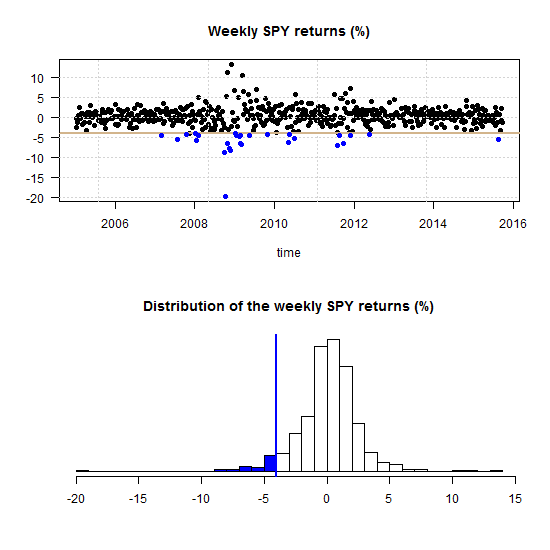
One can ask what is now, given that the market is in the blue region, the probability of a a drawdown in a specific stock?
Multivariate volatility forecasting (4), factor models
To be instructive, I always use very few tickers to describe how a method works (and this tutorial is no different). Most of the time is spent on methods that we can easily scale up. Even if exemplified using only say 3 tickers, a more realistic 100 or 500 is not an obstacle. But, is it really necessary to model the volatility of each ticker individually? No.
If we want to forecast the covariance matrix of all components in the Russell 2000 index we don’t leave much on the table if we model only a few underlying factors, much less than 2000.
Volatility factor models are one of those rare cases where the appeal is both theoretical and empirical. The idea is to create a few principal components and, under the reasonable assumption that they drive the bulk of comovement in the data, model those few components only.
Multivariate volatility forecasting (3), Exponentially weighted model
Broadly speaking, complex models can achieve great predictive accuracy. Nonetheless, a winner in a kaggle competition is required only to attach a code for the replication of the winning result. She is not required to teach anyone the built-in elements of his model which gives the specific edge over other competitors. In a corporation settings your manager and his manager and so forth MUST feel comfortable with the underlying model. Mumbling something like “This artificial-neural-network is obtained by using a grid search over a range of parameters and connection weights where the architecture itself is fixed beforehand…”, forget it!