Another opinion piece.
If you can’t explain it simply you don’t understand it well enough.
(Albert Einstein)
Another opinion piece.
If you can’t explain it simply you don’t understand it well enough.
(Albert Einstein)
The term mutual information is drawn from the field of information theory. Information theory is busy with the quantification of information. For example, a central concept in this field is entropy, which we have discussed before.
If you google the term “mutual information” you will land at some page which if you understand it, there would probably be no need for you to google it in the first place. For example:
Not limited to real-valued random variables and linear dependence like the correlation coefficient, mutual information (MI) is more general and determines how different the joint distribution of the pair (X,Y) is to the product of the marginal distributions of X and Y. MI is the expected value of the pointwise mutual information (PMI).
which makes sense at first read only for those who don’t need to read it. It’s the main motivation for this post: to provide a clear intuition behind the pointwise mutual information term and equations, for everyone. At the end of this page, you would understand what mutual information metric actually measures, and how you should interpret it. We start with the easier concept of conditional probability and work our way through to the concept of pointwise mutual information.
Principal component analysis (PCA) is one of the earliest multivariate techniques. Yet not only it survived but it is arguably the most common way of reducing the dimension of multivariate data, with countless applications in almost all sciences.
Mathematically, PCA is performed via linear algebra functions called eigen decomposition or singular value decomposition. By now almost nobody cares how it is computed. Implementing PCA is as easy as pie nowadays- like many other numerical procedures really, from a drag-and-drop interfaces to prcomp in R or from sklearn.decomposition import PCA in Python. So implementing PCA is not the trouble, but some vigilance is nonetheless required to understand the output.
This post is about understanding the concept of variance explained. With the risk of sounding condescending, I suspect many new-generation statisticians/data-scientists simply echo what is often cited online: “the first principal component explains the bulk of the movement in the overall data” without any deep understanding. What does “explains the bulk of the movement in the overall data” mean exactly, actually?
Moving average is one of the most commonly used smoothing method, basically the go-to. It helps us detect trend in the data by smoothing out short term fluctuations. The computation is trivial: take the most recent k points and simple-average them. Here is how it looks:
Many years ago, when I was still trying to beat the market, I used to pair-trade. In principle it is quite straightforward to estimate the correlation between two stocks. The estimator for beta is very important since it determines how much you should long the one and how much you should short the other, in order to remain market-neutral. In practice it is indeed very easy to estimate, but I remember I never felt genuinely comfortable with the results. Not only because of instability over time, but also because the Ordinary Least Squares (OLS from here on) estimator is theoretically justified based on few text-book assumptions, most of which are improper in practice. In addition, the OLS estimator it is very sensitive to outliers. There are other good alternatives. I have described couple of alternatives here and here. Here below is another alternative, provoked by a recent paper titled Adaptive Huber Regression.
This post is about the concept of entropy in the context of information-theory. Where does the term entropy comes from? What does it actually mean? And how does it clash with the notion of robustness?
This post provides an intuitive explanation for the term Latent Variable.
Broadly speaking, we can classify financial markets conditions into two categories: Bull and Bear. The first is a “todo bien” market, tranquil and generally upward sloping. The second describes a market with a downturn trend, usually more volatile. It is thought that those bull\bear terms originate from the way those animals supposedly attack. Bull thrusts its horns up while a bear swipe its paws down. At any given moment, we can only guess the state in which we are in, there is no way of telling really; simply because those two states don’t have a uniformly exact definitions. So basically we never actually observe a membership of an observation. In this post we are going to use (finite) mixture models to try and assign daily equity returns to their bull\bear subgroups. It is essentially an unsupervised clustering exercise. We will create our own recession indicator to help us quantify if the equity market is contracting or not. We use minimal inputs, nothing but equity return data. Starting with a short description of Finite Mixture Models and moving on to give a hands-on practical example.
Are returns this year actually different than what can be expected from a typical year? Is the variance actually different than what can be expected from a typical year? Those are fairly light, easy to answer questions. We can use tests for equality of means or equality of variances.
But how about the following question:
is the profile\behavior of returns this year different than what can be expected in a typical year?
This is a more general and important question, since it encompasses all moments and tail behavior. And it is not as trivial to answer.
In this post I am scratching an itch I had since I wrote Understanding Kullback – Leibler Divergence. In the Kullback – Leibler Divergence post we saw how to quantify the difference between densities, exemplified using SPY return density per year. Once I was done with that post I was thinking there must be a way to test the difference formally, rather than just quantify, visualize and eyeball. And indeed there is. This post aim is to show to formally test for equality between densities.
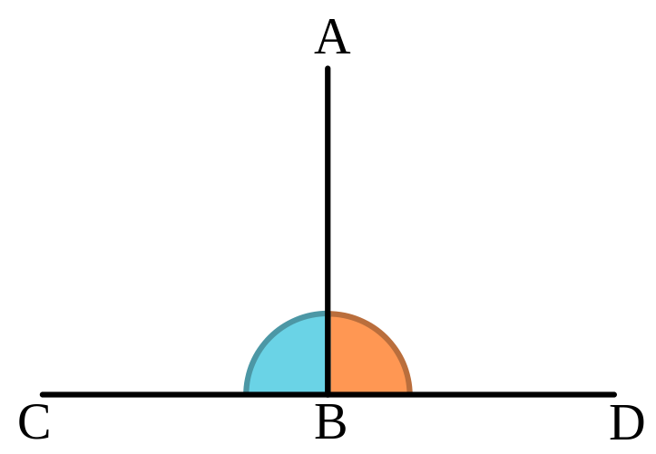
The word Orthogonality originates from a combination of two words in ancient Greek: orthos (upright), and gonia (angle). It has a geometrical meaning. It means two lines create a 90 degrees angle between them. So one line is perpendicular to the other line. Like so:
Even though Orthogonality is a geometrical term, it appears very often in statistics. You probably know that in a statistical context orthogonality means uncorrelated, or linearly independent. But why?
Why use a geometrical term to describe a statistical relation between random variables? By extension, why does the word angle appears in the incredibly common regression method least-angle regression (LARS)? Enough losing sleep over it (as you undoubtedly do), an extensive answer below.
I recently spotted the following intriguing paper: Market intraday momentum.
From the abstract of that paper:
Based on high frequency S&P 500 exchange-traded fund (ETF) data from 1993–2013, we show an intraday momentum pattern: the first half-hour return on the market as measured from the previous day’s market close predicts the last half-hour return. This predictability, which is both statistically and economically significant is stronger on more volatile days, on higher volume days, on recession days, and on major macroeconomic news release days.
Nice! Looks like we can all become rich now. I mean, given how it’s written, it should be quite easy for any individual with a trading account and a mouse to leverage up and start accumulating. Maybe this is so, but let’s have an informal closer look, with as little effort as possible, and see if there is anything we can say about this idea.
Higher moments such as Skewness and Kurtosis are not as explored as they should be.
These moments are crucial for managing portfolio risk. At least as important as volatility, if not more. Skewness relates to asymmetry risk and Kurtosis relates to tail risk.
Despite their great importance, those higher moments enjoy only a small portion of attention compared with their lower more friendly moments: the mean and the variance. In my opinion, one reason for this may be the impossibility of estimating those moments, estimating them accurately that is.
It is yet another situation where Curse of Dimensonality rears its enchanting head (and an idea for a post is born..).
It is easy to measure distance between two points. But what about measuring distance between two distributions? Good question. Long answer. Welcome the Kullback – Leibler Divergence measure.
The motivation for thinking about the Kullback – Leibler Divergence measure is that you can pick up questions such as: “how different was the behavior of the stock market this year compared with the average behavior?”. This is a rather different question than the trivial “how was the return this year compared to the average return?”.
Shrinkage in statistics has increased in popularity over the decades. Now statistical shrinkage is commonplace, explicitly or implicitly.
But when is it that we need to make use of shrinkage? At least partly it depends on signal-to-noise ratio.
In statistics, outliers are as thorny topic as it gets. Is it legitimate to treat the observations seen during global financial crisis as outliers? or are those simply a feature of the system, and as such are integral part of a very fat tail distribution?