Broadly speaking, complex models can achieve great predictive accuracy. Nonetheless, a winner in a kaggle competition is required only to attach a code for the replication of the winning result. She is not required to teach anyone the built-in elements of his model which gives the specific edge over other competitors. In a corporation settings your manager and his manager and so forth MUST feel comfortable with the underlying model. Mumbling something like “This artificial-neural-network is obtained by using a grid search over a range of parameters and connection weights where the architecture itself is fixed beforehand…”, forget it!
Your audience needs to understand, and understand fast. They don’t have the will or time to pick up on anything too tedious, even if it can be slightly more accurate. Simplicity is a very important model-selection criterion in business. In multivariate volatility estimation, the simplest way is to use the historical covariance matrix. But it is too simple, we already know volatility is time-varying. You often see practitioners use rolling standard deviation as a way to model time-varying volatility. It may be less accurate than other state-of-the-art methods like Range-based Covariance Estimation but it is very simple to implement and easy to explain.
This is where exponentially weighted covariance estimation steps in. What is a rolling window estimation if not an equally weighted of the past within the window and zero weight outside of the window. If we have a vector of 5 observation and we use a window of 2 than the vector of weights for estimation is [0,0,0,0.5,0.5]. A step further is to give at least some weight to a more distant past, but also to weight more heavily the most recent observations, say the weight vector [0.05, 0.1, 0.15, 0.3, 0.4]. This simple idea of weights which are decaying to zero as the past becomes past is old yet still prosperous in time series literature.
In accordance with the stylized fact that low volatility follow low volatility and high volatility follow high volatility (volatility clustering), this idea is perfectly suited for multivariate volatility forecasting. Consider the following:
(1) 
where  is the current estimate of the covariance matrix, and
  is the covariance matrix based on the past up until the period t-1. Another interpretation I carry is that we use the simplest estimate possible which is the historical covariance matrix, but adding some weight (
 , to be exact) to a covariance matrix estimated based on only the most recent observation. This is really easy to explain which makes it very popular, an industry standard almost. We can estimate how fast we would like the weights to decline, but you can also use some previous research which estimates the decaying parameter as 0.94.
A function written by Eric Zivot does all the work for us (scroll down for the function’s code). See how it looks, I use the same data as in my previous posts and plot the correlation matrix over time for a couple of different lambda values:
|
1 2 3 4 5 6 7 8 9 10 11 12 13 14 15 16 17 18 19 20 21 22 23 24 25 26 27 28 29 30 31 32 |
library(quantmod) k <- 10 # how many years back? end<- format(Sys.Date(),"%Y-%m-%d") start<-format(Sys.Date() - (k*365),"%Y-%m-%d") sym = c('SPY', 'TLT', 'IEF') l <- length(sym) dat0 = getSymbols(sym[1], src="yahoo", from=start, to=end, auto.assign = F, warnings = FALSE, symbol.lookup = F) n = NROW(dat0) dat = array(dim = c(n,NCOL(dat0),l)) ; ret = matrix(nrow = n, ncol = l) for (i in 1:l){ dat0 = getSymbols(sym[i], src="yahoo", from=start, to=end, auto.assign = F, warnings = FALSE, symbol.lookup = F) dat[1:n,,i] = dat0 ret[2:n,i] = (dat[2:n,4,i]/dat[1:(n-1),4,i] - 1) # returns, close to close, percent } ret <- 100*na.omit(ret)# Remove the first observation time <- index(dat0)[-1] colnames(ret) <- sym nassets <- dim(ret)[2] TT <- dim(ret)[1] tail(ret) cor_mat <- covEWMA(as.data.frame(ret), lambda=.95, return.cor=T) dim(cor_mat) plot(cor_mat[,1,2]~time, ty = "l", las = 1, ylim = c(-1,1), main = "lambda= 0.95") ; grid() lines(cor_mat[,1,3]~time, col = 2); lines(cor_mat[,2,3]~time, col = 3) leg <- c(paste(sym[1], "with", sym[2]) , paste(sym[1], "with", sym[3]), paste(sym[2], "with", sym[3])) legend("bottomleft",leg, col=1:3, lwd=lwd1, cex=.8, bty="n",text.col=1:3) |
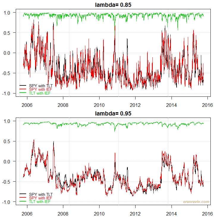
You can see that if you assign 15% weight for the last observation you get somewhat volatile estimates. A weight of only 5% (lambda = 0.95) gives a smoother estimate, but perhaps less accurate.
Apart from the simplicity, another important advantage is that there is no need to care about invertability, since at each point in time the estimate is simply a weighted average of two valid correlation matrices (see post number (1) for more information on that). And also, you can apply this method to whatever financial instrument, liquid or illiquid, which is another reason for it being so popular.
|
1 2 3 4 5 6 7 8 9 10 11 12 13 14 15 16 17 18 19 20 21 22 23 24 25 26 27 28 29 30 31 32 33 34 35 36 37 38 39 40 41 42 43 44 45 46 47 |
From Eric Zivot: http://faculty.washington.edu/ezivot covEWMA <- function(factors, lambda=0.96, return.cor=FALSE) { ## Inputs: ## factors N x K numerical factors data. data is class data.frame ## N is the time length and K is the number of the factors. ## lambda scalar. exponetial decay factor between 0 and 1. ## return.cor Logical, if TRUE then return EWMA correlation matrices ## Output: ## covEWMA array. dimension is N x K x K. if (is.data.frame(factors)){ factor.names = colnames(factors) t.factor = nrow(factors) k.factor = ncol(factors) factors = as.matrix(factors) t.names = rownames(factors) } else { stop("factor data should be saved in data.frame class.") } if (lambda>=1 || lambda <= 0){ stop("exponential decay value lambda should be between 0 and 1.") } else { cov.f.ewma = array(,c(t.factor,k.factor,k.factor)) cov.f = var(factors) # unconditional variance as EWMA at time = 0 mfactors <- apply(factors,2, mean) FF = (factors[1,]- mfactors) %*% t(factors[1,]- mfactors) cov.f.ewma[1,,] = (1-lambda)*FF + lambda*cov.f for (i in 2:t.factor) { FF = (factors[i,]- mfactors) %*% t(factors[i,]- mfactors) cov.f.ewma[i,,] = (1-lambda)*FF + lambda*cov.f.ewma[(i-1),,] } } dimnames(cov.f.ewma) = list(t.names, factor.names, factor.names) if(return.cor) { cor.f.ewma = cov.f.ewma for (i in 1:dim(cor.f.ewma)[1]) { cor.f.ewma[i, , ] = cov2cor(cov.f.ewma[i, ,]) } return(cor.f.ewma) } else{ return(cov.f.ewma) } } |
References
Forecasting with Exponential Smoothing: The State Space Approach (Springer Series in Statistics)
UPDATE on 2015-Oct-14:
An astute reader rightly commented that the function is not suitable for out-of-sample prediction, this is correct. The reason is that we shrink towards the sample covariance matrix which is based on the full sample, which we don’t yet know before the sample ends. In a realistic settings we can only use information available up to that point where we wish to predict. Subsequently, I altered the original function to include an one extra parameter (the initial window length for estimation of the covariance matrix). The initial covariance matrix is then taken only using information up to the time the prediction is made, as is the scaling. The figures do not change much. The new modified function is below
|
1 2 3 4 5 6 7 8 9 10 11 12 13 14 15 16 17 18 19 20 21 22 23 24 25 26 27 28 29 30 31 32 33 34 35 36 37 38 39 40 41 42 43 44 45 46 47 48 |
covEWMAoos <- function(factors, lambda=0.96, return.cor=FALSE, wind = 30) { # based on the function covEWMA written by Eric Zivot # Adjusted for out-of-sample covariance prediction ## Inputs: ## factors N x K numerical factors data. data is class data.frame ## N is the time length and K is the number of the factors. ## lambda scalar. exponetial decay factor between 0 and 1. ## return.cor Logical, if TRUE then return EWMA correlation matrices ## Output: ## cov.f.ewma array. dimension is N x K x K. ## wind Saclar. The initial window length if (is.data.frame(factors)){ factor.names = colnames(factors) t.factor = nrow(factors) k.factor = ncol(factors) factors = as.matrix(factors) t.names = rownames(factors) } else { stop("factor data should be saved in data.frame class.") } if (lambda>=1 || lambda <= 0){ stop("exponential decay value lambda should be between 0 and 1.") } else { cov.f.ewma = array(,c(t.factor,k.factor,k.factor)) mfactors <- apply(factors[1:(wind-1),], 2, mean) FF = (factors[(wind-1),]- mfactors) %*% t(factors[(wind-1), ]- mfactors) cov.f = var(factors[1:(wind-1),]) cov.f.ewma[(wind-1),,] = (1-lambda)*FF + lambda*cov.f for (i in wind : t.factor) { cov.f = var(factors[1:i,]) # unconditional variance up to t. mfactors <- apply(factors[1:i,], 2, mean) FF = (factors[i,]- mfactors) %*% t(factors[i,]- mfactors) cov.f.ewma[i,,] = (1-lambda)*FF + lambda*cov.f.ewma[(i-1),,] } } dimnames(cov.f.ewma) = list(t.names, factor.names, factor.names) if(return.cor) { cor.f.ewma = cov.f.ewma for (i in wind:dim(cor.f.ewma)[1]) { cor.f.ewma[i, , ] = cov2cor(cov.f.ewma[i, ,]) } return(cor.f.ewma) }else{ return(cov.f.ewma) } } |


Eran,
Is this method an online and vectorized method? Because I don’t see you calling a for loop beyond getting the instruments. Is this output something that can be used for a rolling backtest?
-Ilya
Hi Ilya, updated.